Databases and dbplyr and SQL, oh my!

Jo Hardin

2024-01-08

Course logistics

https://sds261-sql.netlify.app/

syllabus
class notes
clicker questions
project
getting started with GitHub

SQL:Structured Query Language

What is a database?

structured collection of data organized with
- efficient storage
- easy retrieval
- consistent management
data stored in tables which are linked to one another via keys

Tidy data

data frame (R) or table (SQL)
columns of variables
rows of observational units

Differences between R and SQL

tables in SQL databases can be arbitrarily large
- live in storage, computer’s hard drive (usually remote)
data frames in R
- live in memory (RAM) on your personal computer
tables in a database are linked via a key.

Today’s example

The `airlines` database

Consider a database of US flights between 2010 and 2017. The flights are downloaded from the Bureau of Transportation Statistics, US Department of Transportation. The database is a superset of the nycflights13 R package that tracks only flights in and out of airports serving New York City in 2013.

SQL connection

To set up a SQL connection, you need the location of the server (host) as well as a username and password.

con_air <- DBI::dbConnect(
  RMariaDB::MariaDB(),
  dbname = "airlines",
  host = Sys.getenv("MDSR_HOST"),
  user = Sys.getenv("MDSR_USER"),
  password = Sys.getenv("MDSR_PWD")
)

Hadley Wickham discusses how to use Sys.getenv: https://cran.r-project.org/web/packages/httr/vignettes/secrets.html

Tables in `airlines` database

DBI::dbListTables(con_air)

[1] "airports" "carriers" "flights"  "planes"

SQL tables as `tbl`

carriers <- dplyr::tbl(con_air, "carriers")
dim(carriers)

[1] NA  2

head(carriers)

# Source:   SQL [6 x 2]
# Database: mysql  [mdsr_public@mdsr.cdc7tgkkqd0n.us-east-1.rds.amazonaws.com:NA/airlines]
  carrier name                         
  <chr>   <chr>                        
1 02Q     Titan Airways                
2 04Q     Tradewind Aviation           
3 05Q     Comlux Aviation, AG          
4 06Q     Master Top Linhas Aereas Ltd.
5 07Q     Flair Airlines Ltd.          
6 09Q     Swift Air, LLC

SQL tables as `tibble`

The function collect() copies a SQL table from it’s server location on disk to your local memory location in R.

carriers_tibble <- carriers |>
  dplyr::collect()

dim(carriers_tibble)

[1] 1610    2

head(carriers_tibble)

# A tibble: 6 × 2
  carrier name                         
  <chr>   <chr>                        
1 02Q     Titan Airways                
2 04Q     Tradewind Aviation           
3 05Q     Comlux Aviation, AG          
4 06Q     Master Top Linhas Aereas Ltd.
5 07Q     Flair Airlines Ltd.          
6 09Q     Swift Air, LLC

How much space does `carriers` take up?

The data frame in R takes up 2 orders of magnitude of memory more than the table which just points to the object in SQL.

carriers |>
  object.size() |>
  print(units = "Kb")

5.2 Kb

carriers_tibble |>
  object.size() |>
  print(units = "Kb")

234.8 Kb

What is SQL?

SQL is a programming language for working with relational databases.
SQL has been around since the 1970s, but has, unfortunately, many different dialects.
To connect to the Smith and mdsr databases (via R and DBeaver), we will use MySQL.
To connect to DuckDB, we will use the dialect native to DuckDB.

Using SQL in RStudio

We will write SQL code in three distinct ways:

Using the package dbplyr R will directly translate dplyr code into SQL.
Using the DBI package, we can send SQL queries through an r chunk.
Using a sql chunk, we can write actual SQL code inside a quarto document.

1. Translating dplyr code into SQL

The function dbListTables() in the DBI package will tell us what tables exist in the airlines database.

DBI::dbListTables(con_air)

[1] "airports" "carriers" "flights"  "planes"

flights <- dplyr::tbl(con_air, "flights")
carriers <- dplyr::tbl(con_air, "carriers")

1. Translating dplyr code into SQL

Over what years is the flights data taken?

yrs <- flights |>
  summarize(min_year = min(year), max_year = max(year))

yrs

# Source:   SQL [1 x 2]
# Database: mysql  [mdsr_public@mdsr.cdc7tgkkqd0n.us-east-1.rds.amazonaws.com:NA/airlines]
  min_year max_year
     <int>    <int>
1     2010     2017

1. Translating dplyr code into SQL

Because flights is not actually a data.frame in R (but instead a tbl in SQL), the work that was done above was actually performed in SQL. To see the SQL code, we can use the function show_query.

dplyr::show_query(yrs)

<SQL>
SELECT MIN(`year`) AS `min_year`, MAX(`year`) AS `max_year`
FROM `flights`

1. Translating dplyr code into SQL

Create a data set containing only flights between LAX and BOS in 2012.

la_bos <- flights |>
  filter(year == 2012 & ((origin == "LAX" & dest == "BOS") | 
           (origin == "BOS" & dest == "LAX"))) 

dplyr::show_query(la_bos)

<SQL>
SELECT *
FROM `flights`
WHERE (`year` = 2012.0 AND ((`origin` = 'LAX' AND `dest` = 'BOS') OR (`origin` = 'BOS' AND `dest` = 'LAX')))

1. Translating dplyr code into SQL

dbplyr doesn’t translate every R command into SQL.
SQL is not a statistical software and doesn’t, for example, have a mechanism for creating data visualizations.
track which R commands are connected to SQL at the dbplyr reference sheet.

2. SQL queries via the DBI package

Look at the first few rows of the flights data.

DBI::dbGetQuery(con_air,
                "SELECT * FROM flights LIMIT 8;")

  year month day dep_time sched_dep_time dep_delay arr_time sched_arr_time
1 2010    10   1        1           2100       181      159           2320
2 2010    10   1        1           1920       281      230           2214
3 2010    10   1        3           2355         8      339            334
4 2010    10   1        5           2200       125       41           2249
5 2010    10   1        7           2245        82      104           2347
6 2010    10   1        7             10        -3      451            500
7 2010    10   1        7           2150       137      139           2337
8 2010    10   1        8             15        -7      538            537
  arr_delay carrier tailnum flight origin dest air_time distance cancelled
1       159      XE  N11137   2558    EWR  OMA      162     1133         0
2       256      B6  N659JB    562    FLL  SWF      131     1119         0
3         5      B6  N563JB    701    JFK  SJU      196     1597         0
4       112      XE  N16559   5982    IAD  BNA       82      542         0
5        77      OO  N908SW   6433    LAX  FAT       37      209         0
6        -9      AA  N3FRAA    700    LAX  DFW      150     1235         0
7       122      DL  N347NW   1752    ATL  IAD       70      533         0
8         1      CO  N73283   1740    SMF  IAH      193     1609         0
  diverted hour minute           time_hour
1        0   21      0 2010-10-01 21:00:00
2        0   19     20 2010-10-01 19:20:00
3        0   23     55 2010-10-01 23:55:00
4        0   22      0 2010-10-01 22:00:00
5        0   22     45 2010-10-01 22:45:00
6        0    0     10 2010-10-01 00:10:00
7        0   21     50 2010-10-01 21:50:00
8        0    0     15 2010-10-01 00:15:00

2. SQL queries via the DBI package

How many flights per year are in the flights table?

DBI::dbGetQuery(con_air, 
  "SELECT year, count(*) AS num_flights FROM flights GROUP BY year ORDER BY num_flights;")

  year num_flights
1 2016     5617658
2 2017     5674621
3 2015     5819079
4 2014     5819811
5 2011     6085281
6 2012     6096762
7 2013     6369482
8 2010     6450117

3. Direct SQL queries via `sql` chunks

SQL queries can be written directly inside a sql chunk in RStudio.

```{sql}
#| connection: con_air

SELECT * FROM flights LIMIT 8;
```

8 records
year	month	day	dep_time	sched_dep_time	dep_delay	arr_time	sched_arr_time	arr_delay	carrier	tailnum	flight	origin	dest	air_time	distance	hour	minute	time_hour
2010	10	1	1	2100	181	159	2320	159	XE	N11137	2558	EWR	OMA	162	1133	21	0	2010-10-01 21:00:00
2010	10	1	1	1920	281	230	2214	256	B6	N659JB	562	FLL	SWF	131	1119	19	20	2010-10-01 19:20:00
2010	10	1	3	2355	8	339	334	5	B6	N563JB	701	JFK	SJU	196	1597	23	55	2010-10-01 23:55:00
2010	10	1	5	2200	125	41	2249	112	XE	N16559	5982	IAD	BNA	82	542	22	0	2010-10-01 22:00:00
2010	10	1	7	2245	82	104	2347	77	OO	N908SW	6433	LAX	FAT	37	209	22	45	2010-10-01 22:45:00
2010	10	1	7	10	-3	451	500	-9	AA	N3FRAA	700	LAX	DFW	150	1235	0	10	2010-10-01 00:10:00
2010	10	1	7	2150	137	139	2337	122	DL	N347NW	1752	ATL	IAD	70	533	21	50	2010-10-01 21:50:00
2010	10	1	8	15	-7	538	537	1	CO	N73283	1740	SMF	IAH	193	1609	0	15	2010-10-01 00:15:00

3. Direct SQL queries via `sql` chunks

SQL queries can be written directly inside a sql chunk in RStudio.

```{sql}
#| connection: con_air

SELECT year, count(*) AS num_flights 
       FROM flights 
       GROUP BY year 
       ORDER BY num_flights;
```

8 records
year	num_flights
2016	5617658
2017	5674621
2015	5819079
2014	5819811
2011	6085281
2012	6096762
2013	6369482
2010	6450117

Good practice

Always a good idea to terminate the SQL connection when you are done with it.

dbDisconnect(con_air, shutdown = TRUE)

Using SQL in DBeaver

DBeaver is a free SQL client that supports MySQL
writing SQL code in R has some benefits (e.g., piping results tables into ggplot2 for visualizations)
using a SQL client that is designed for SQL queries has benefits as well.
to use DBeaver, download the client onto your computer and open it from your Applications.

Tools: GitHub

Lab assignments are submitted via GitHub
Follow Jenny Bryan’s advice on how to get GitHub set-up: http://happygitwithr.com/
Follow course specific advice: https://sds261-sql.netlify.app/github

Steps for weekly homework

Receive a link to the new assignment (clicking on the link will create a new private repo)
Use RStudio
- New Project, version control, Git
- Clone the repo using SSH
Create a new file sds261-lab#-lname-fname.qmd. (If the .qmd file already exists, rename the file to sds261-lab#-lname-fname.qmd.)
Do the assignment
- commit and push after every problem
For work done in DBeaver (.sql files), use the same naming convention: sds261-lab#-lname-fname.sql.
All necessary files must be in the same folder (e.g., data, .sql files, etc.)

A GitHub merge conflict

On GitHub (on the web) edit the README document and Commit it with a message describing what you did.
Then, in RStudio also edit the README document with a different change.
- Commit your changes
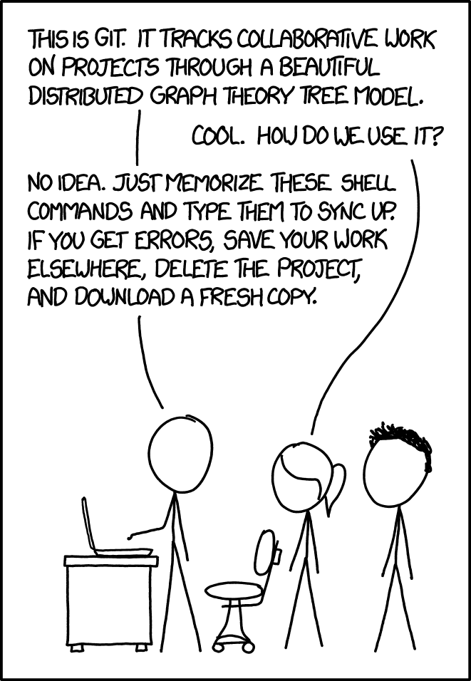
- Try to push – you’ll get an error!
- Try pulling
- Resolve the merge conflict and then commit and push
As you work in teams you are likely to run into merge conflicts, learning how to resolve them properly will be very important.

Databases and dbplyr and SQL, oh my!

Course logistics

SQL:Structured Query Language

What is a database?

Tidy data

Differences between R and SQL

Today’s example

The airlines database

SQL connection

Tables in airlines database

SQL tables as tbl

SQL tables as tibble

How much space does carriers take up?

What is SQL?

Using SQL in RStudio

1. Translating dplyr code into SQL

1. Translating dplyr code into SQL

1. Translating dplyr code into SQL

1. Translating dplyr code into SQL

1. Translating dplyr code into SQL

2. SQL queries via the DBI package

2. SQL queries via the DBI package

3. Direct SQL queries via sql chunks

3. Direct SQL queries via sql chunks

Good practice

Using SQL in DBeaver

Tools: GitHub

Steps for weekly homework

A GitHub merge conflict

GitHub

The `airlines` database

Tables in `airlines` database

SQL tables as `tbl`

SQL tables as `tibble`

How much space does `carriers` take up?

3. Direct SQL queries via `sql` chunks

3. Direct SQL queries via `sql` chunks