Data Science, the SQL

Back to the flights

The examples below use the airlines database, including the flights, carriers, airports, and planes tables.

Efficiencies

Reconsider this analogy:

Each library (database) has books (tables). Each book (table) has pages (rows). Each page (row) has a unique page number to identify it (key value); to find a particular page, you sort through the page numbers (key values). But it isn’t immediately obvious where the particular page of interest is, you might have to page through the book a little bit to find the page of interest. It would be easier if you had several bookmarks throughout the book to anchor some of the page numbers. For example, if you want page 1047 and you have a bookmark on page 1050, you only have to turn back three pages. The bookmark is an index, it helps you find the desired rows much more quickly.¹

`KEY`s

Keys are unique identifiers for each row, used primarily for connecting tables. Keys are generally not helpful for efficiency, but they are important for data integrity and relationships between tables. A key is a pointer that identifies a record. In practice, a key is one or more columns that are earmarked to uniquely identify a record in a table. Keys serve two main purposes:

They provide constraints on the column such as that it can’t store duplicate or null values.
They are also used to generate relationships among different tables.

`INDEX`es

By indexing the rows, SQL is able to optimize sorting and joining tables.
The index is created in advance (when the table is created) and saved to disk, which can take up substantial space on the disk.
Sometimes more than one variable is used to index the table.
There are trade-offs to having a lot of indexes (disk space but fast wrangling) versus a few indexes (slow wrangling but less space).
A table may have more than one index but you shouldn’t add indexes to every column in a table, as these have to be updated for every addition/update/delete to the column.
Indexes should be added to columns that are frequently included in queries.

`SHOW INDEXES`

Notice that the planes table has a single PRIMARY key. That primary key is used to index the table. The flights table has no PRIMARY key, but it does have six different indexes: Year, Date, Origin, Dest, Carrier, and tailNum.

SHOW INDEXES FROM planes;

1 records
Table	Non_unique	Key_name	Seq_in_index	Column_name	Collation	Cardinality	Sub_part	Packed	Null	Index_type	Comment	Index_comment
planes	0	PRIMARY	1	tailnum	A	3322				BTREE

SHOW INDEXES FROM flights;

8 records
Table	Non_unique	Key_name	Seq_in_index	Column_name	Collation	Cardinality	Null	Index_type
flights	1	Year	1	year	A	7	YES	BTREE
flights	1	Date	1	year	A	7	YES	BTREE
flights	1	Date	2	month	A	89	YES	BTREE
flights	1	Date	3	day	A	2712	YES	BTREE
flights	1	Origin	1	origin	A	2267		BTREE
flights	1	Dest	1	dest	A	2267		BTREE
flights	1	Carrier	1	carrier	A	134		BTREE
flights	1	tailNum	1	tailnum	A	37862	YES	BTREE

`SHOW INDEXES`

The values output by SHOW INDEXES are:¹

Table: The name of the table.
Non_unique: 0 if the index cannot contain duplicates, 1 if it can.
Key_name: The name of the index. If the index is the primary key, the name is always PRIMARY.
Seq_in_index: The column sequence number in the index, starting with 1.
Column_name: The column name. See also the description for the Expression column.
Collation: How the column is sorted in the index. This can have values A (ascending), D (descending), or NULL (not sorted).
Cardinality: An estimate of the number of unique values in the index.
Sub_part: The index prefix. That is, the number of indexed characters if the column is only partly indexed, NULL if the entire column is indexed.
Packed: Indicates how the key is packed. NULL if it is not.
Null: Contains YES if the column may contain NULL values and ’’ if not.
Index_type: The index method used (BTREE, FULLTEXT, HASH, RTREE).
Comment: Information about the index not described in its own column, such as disabled if the index is disabled.
Index_comment: Any comment provided for the index with a COMMENT attribute when the index was created.

Partitioning

Another way to speed up query retrievals is to partition the data tables. If, for example, the SNL queries were always done by year, then the episodes table could be partitioned such that they are stored as separate tables (one per year). The partitioning functions as an index on year. The user would not be able to tell the difference between the unpartitioned episodes table and the partitioned one. However, queries done by year would be faster. Queries done grouped in another way would be slower.

Querying quickly

Indexes are built to accommodate the specific queries that are most likely to be run. However, you might not know which queries are going to be run, so it isn’t always obviously how to index a table.

SHOW INDEXES FROM flights;

8 records
Table	Non_unique	Key_name	Seq_in_index	Column_name	Collation	Cardinality	Null	Index_type
flights	1	Year	1	year	A	7	YES	BTREE
flights	1	Date	1	year	A	7	YES	BTREE
flights	1	Date	2	month	A	89	YES	BTREE
flights	1	Date	3	day	A	2712	YES	BTREE
flights	1	Origin	1	origin	A	2267		BTREE
flights	1	Dest	1	dest	A	2267		BTREE
flights	1	Carrier	1	carrier	A	134		BTREE
flights	1	tailNum	1	tailnum	A	37862	YES	BTREE

`EXPLAIN` with `distance`

EXPLAIN communicates how onerous the query is, without actually running it—saving you the time of having to wait for it to execute.

EXPLAIN SELECT * FROM flights WHERE distance > 3000;

1 records
id	select_type	table	partitions	type	possible_keys	key	key_len	ref	rows	filtered	Extra
1	SIMPLE	flights	p1,p2,p3,p4,p5,p6,p7,p8,p9,p10,p11,p12,p13,p14,p15,p16,p17,p18,p19,p20,p21,p22,p23,p24,p25,p26,p27,p28,p29,p30,p31,p32	ALL					47932811	33.3	Using where

If we were to run a query for long flights using the distance column the server will have to inspect each of the 48 million rows, because distance is not indexed. A query on a non-indexed variable is the slowest possible search and is often called a table scan. The 48 million number that you see in the rows column is an estimate of the number of rows that MySQL will have to consult in order to process your query. In general, more rows mean a slower query.

`EXPLAIN` with `year`

A search for recent flights using the year column, which has an index built on it, considers many fewer rows (about 6.3 million, those flights in 2013).

EXPLAIN SELECT * FROM flights WHERE year = 2013;

1 records
id	select_type	table	partitions	type	possible_keys	key	key_len	ref	rows	filtered	Extra
1	SIMPLE	flights	p27	ALL	Year,Date				6369482	100	Using where

`Cardinality` x `rows`

The Cardinality from SHOW INDEXES times the rows from EXPLAIN is roughly the total number of rows in the dataframe.

`EXPLAIN` with `year` and `month`

In a search by year and month, SQL uses the Date index. Only 700,000 rows are searched, those in June of 2013.

EXPLAIN SELECT * FROM flights WHERE year = 2013 AND month = 6;

1 records
id	select_type	table	partitions	type	possible_keys	key	key_len	ref	rows	filtered	Extra
1	SIMPLE	flights	p27	ref	Year,Date	Date	6	const,const	714535	100

`EXPLAIN` with `month`

If we search for particular months across all years, the indexing does not help at all. The query results in a table scan.

EXPLAIN SELECT * FROM flights WHERE month = 6;

1 records
id	select_type	table	partitions	type	possible_keys	key	key_len	ref	rows	filtered	Extra
1	SIMPLE	flights	p1,p2,p3,p4,p5,p6,p7,p8,p9,p10,p11,p12,p13,p14,p15,p16,p17,p18,p19,p20,p21,p22,p23,p24,p25,p26,p27,p28,p29,p30,p31,p32	ALL					47932811	10	Using where

Although month is part of the Date index, it is the second column in the index, and thus it doesn’t help us when we aren’t filtering on year. Thus, if it were common for our users to search on month without year, it would probably be worth building an index on month. Were we to actually run these queries, there would be a significant difference in computational time.

`EXPLAIN` with `JOIN` - faster

The cardinality of the index on tailnum is large (the number of rows in flights associated with each unique value of tailnum is small).

EXPLAIN 
  SELECT * FROM planes p 
  LEFT JOIN flights o ON p.tailnum = o.TailNum
  WHERE manufacturer = 'BOEING';

2 records
id	select_type	table	partitions	type	possible_keys	key	key_len	ref	rows	filtered	Extra
1	SIMPLE	p		ALL					3322	10	Using where
1	SIMPLE	o	p1,p2,p3,p4,p5,p6,p7,p8,p9,p10,p11,p12,p13,p14,p15,p16,p17,p18,p19,p20,p21,p22,p23,p24,p25,p26,p27,p28,p29,p30,p31,p32	ref	tailNum	tailNum	9	airlines.p.tailnum	1266	100

`EXPLAIN` with `JOIN` - slower

The cardinality of the index on year is small (the number of rows in flights associated with each unique year is large).

EXPLAIN 
  SELECT * FROM planes p 
  LEFT JOIN flights o ON p.Year = o.Year
  WHERE manufacturer = 'BOEING';

2 records
id	select_type	table	partitions	type	possible_keys	key	key_len	ref	rows	filtered	Extra
1	SIMPLE	p		ALL					3322	10	Using where
1	SIMPLE	o	p1,p2,p3,p4,p5,p6,p7,p8,p9,p10,p11,p12,p13,p14,p15,p16,p17,p18,p19,p20,p21,p22,p23,p24,p25,p26,p27,p28,p29,p30,p31,p32	ref	Year,Date	Year	3	airlines.p.year	6450117	100	Using where

SQL in dbplyr

As mentioned previously, dbplyr doesn’t translate every R command into SQL. After all, SQL is not a statistical software and doesn’t, for example, have a mechanism for creating data visualizations. To track which R commands are connected to SQL see the dbplyr reference sheet.

Median

Let’s start with an example, calculating the median altitude in the airports table.¹

airports <- tbl(con_air, "airports")

head(airports)

# Source:   SQL [6 x 9]
# Database: mysql  [mdsr_public@mdsr.cdc7tgkkqd0n.us-east-1.rds.amazonaws.com:NA/airlines]
  faa   name                           lat   lon   alt    tz dst   city  country
  <chr> <chr>                        <dbl> <dbl> <int> <int> <chr> <chr> <chr>  
1 04G   Lansdowne Airport             41.1 -80.6  1044    -5 A     Youn… United…
2 06A   Moton Field Municipal Airpo…  32.5 -85.7   264    -6 A     Tusk… United…
3 06C   Schaumburg Regional           42.0 -88.1   801    -6 A     Scha… United…
4 06N   Randall Airport               41.4 -74.4   523    -5 A     Midd… United…
5 09J   Jekyll Island Airport         31.1 -81.4    11    -5 A     Jeky… United…
6 0A9   Elizabethton Municipal Airp…  36.4 -82.2  1593    -5 A     Eliz… United…

Median

It looks like show_query() is providing SQL code for calculating the median!

median_query <- airports |>
  summarize(med_alt = median(alt, na.rm = TRUE))

show_query(median_query)

<SQL>
SELECT PERCENTILE_CONT(0.5) WITHIN GROUP (ORDER BY `alt`) AS `med_alt`
FROM `airports`

Median

But when the SQL code is run, it doesn’t seem to work.

SELECT PERCENTILE_CONT(0.5) WITHIN GROUP (ORDER BY `alt`) AS `med_alt`
FROM `airports`;

Error: You have an error in your SQL syntax; check the manual that corresponds to your MySQL server version for the right syntax to use near 'GROUP (ORDER BY `alt`) AS `med_alt`
FROM `airports`' at line 1 [1064]

Median

What happens when we computer the median on the tbl?

airports |>
  summarize(med_alt = median(alt, na.rm = TRUE))

Error in `collect()`:
! Failed to collect lazy table.
Caused by error:
! You have an error in your SQL syntax; check the manual that corresponds to your MySQL server version for the right syntax to use near 'GROUP (ORDER BY `alt`) AS `med_alt`
FROM `airports`
LIMIT 7' at line 1 [1064]

Median

How can the median be calculated in SQL?

SET @row_index := -1;

SELECT AVG(subquery.alt) AS median_value
FROM (
SELECT @row_index:=@row_index + 1 AS row_index, alt
  FROM airports
  ORDER BY alt
) AS subquery
WHERE subquery.row_index IN (FLOOR(@row_index / 2), CEIL(@row_index / 2));

1 records
median_value
476

Median

Let’s break down what the code is doing… First, set the row_index to -1 and iterate through by adding +1 for each row. Then concatenate the row_index information onto our table of interest. (Basically, create a column that gives a row value to the dataset, sorted by altitude.)

SET @row_index := -1;

SELECT @row_index:=@row_index + 1 AS row_index, alt
  FROM airports
  ORDER BY alt
  LIMIT 10;

Displaying records 1 - 10
row_index	alt
0	-54
1	-42
2	0
3	0
4	0
5	0
6	0
7	0
8	0
9	0

Median

Next, filter the data to include only the middle row or two rows.

SET @row_index := -1;

SELECT *
FROM (
SELECT @row_index:=@row_index + 1 AS row_index, alt
  FROM airports
  ORDER BY alt
) AS subquery
WHERE subquery.row_index IN (FLOOR(@row_index / 2), CEIL(@row_index / 2));

2 records
row_index	alt
728	474
729	477

Median

The last step is to average the middle row(s). If only one row is pulled out in the previous query, then only one row will be averaged (which the computer does happily).

SET @row_index := -1;

SELECT AVG(subquery.alt) AS median_value
FROM (
SELECT @row_index:=@row_index + 1 AS row_index, alt
  FROM airports
  ORDER BY alt
) AS subquery
WHERE subquery.row_index IN (FLOOR(@row_index / 2), CEIL(@row_index / 2));

1 records
median_value
476

Median

Take-aways:

dbplyr is not able to translate the median() function into SQL.
The median is actually really hard to calculate! In particular, it is hard to calculate the median in one pass through the data.

`CASE WHEN` and `ifelse()`

Consider the various R functions that create new variables based on an original variable.

airports |>
  mutate(sea = ifelse(alt > 500, "above sea", "near sea")) |>
  head(5)

# Source:   SQL [5 x 10]
# Database: mysql  [mdsr_public@mdsr.cdc7tgkkqd0n.us-east-1.rds.amazonaws.com:NA/airlines]
  faa   name                     lat   lon   alt    tz dst   city  country sea  
  <chr> <chr>                  <dbl> <dbl> <int> <int> <chr> <chr> <chr>   <chr>
1 04G   Lansdowne Airport       41.1 -80.6  1044    -5 A     Youn… United… abov…
2 06A   Moton Field Municipal…  32.5 -85.7   264    -6 A     Tusk… United… near…
3 06C   Schaumburg Regional     42.0 -88.1   801    -6 A     Scha… United… abov…
4 06N   Randall Airport         41.4 -74.4   523    -5 A     Midd… United… abov…
5 09J   Jekyll Island Airport   31.1 -81.4    11    -5 A     Jeky… United… near…

`CASE WHEN` and `ifelse()`

if_query <- airports |>
  mutate(sea = ifelse(alt > 500, "above sea", "near sea"))

show_query(if_query)

<SQL>
SELECT
  *,
  CASE WHEN (`alt` > 500.0) THEN 'above sea' WHEN NOT (`alt` > 500.0) THEN 'near sea' END AS `sea`
FROM `airports`

`CASE WHEN` and `ifelse()`

SELECT *,
CASE WHEN (`alt` > 500.0) THEN 'above sea' WHEN NOT (`alt` > 500.0) THEN 'near sea' END AS `sea`
FROM `airports` 
LIMIT 5;

5 records
faa	name	lat	lon	alt	tz	dst	city	country	sea
04G	Lansdowne Airport	41.1	-80.6	1044	-5	A	Youngstown	United States	above sea
06A	Moton Field Municipal Airport	32.5	-85.7	264	-6	A	Tuskegee	United States	near sea
06C	Schaumburg Regional	42.0	-88.1	801	-6	A	Schaumburg	United States	above sea
06N	Randall Airport	41.4	-74.4	523	-5	A	Middletown	United States	above sea
09J	Jekyll Island Airport	31.1	-81.4	11	-5	A	Jekyll Island	United States	near sea

`CASE WHEN` and `case_when()`

airports |>
  mutate(sea = case_when(
    alt < 500 ~ "near sea",
    alt < 2000 ~ "low alt",
    alt < 3000 ~ "mod alt",
    alt < 5500 ~ "high alt",
    alt > 5500 ~ "extreme alt")) |>
  head(5)

# Source:   SQL [5 x 10]
# Database: mysql  [mdsr_public@mdsr.cdc7tgkkqd0n.us-east-1.rds.amazonaws.com:NA/airlines]
  faa   name                     lat   lon   alt    tz dst   city  country sea  
  <chr> <chr>                  <dbl> <dbl> <int> <int> <chr> <chr> <chr>   <chr>
1 04G   Lansdowne Airport       41.1 -80.6  1044    -5 A     Youn… United… low …
2 06A   Moton Field Municipal…  32.5 -85.7   264    -6 A     Tusk… United… near…
3 06C   Schaumburg Regional     42.0 -88.1   801    -6 A     Scha… United… low …
4 06N   Randall Airport         41.4 -74.4   523    -5 A     Midd… United… low …
5 09J   Jekyll Island Airport   31.1 -81.4    11    -5 A     Jeky… United… near…

`CASE WHEN` and `case_when()`

cw_query <- airports |>
  mutate(sea = case_when(
    alt < 500 ~ "near sea",
    alt < 2000 ~ "low alt",
    alt < 3000 ~ "mod alt",
    alt < 5500 ~ "high alt",
    alt > 5500 ~ "extreme alt"))

show_query(cw_query)

<SQL>
SELECT
  *,
  CASE
WHEN (`alt` < 500.0) THEN 'near sea'
WHEN (`alt` < 2000.0) THEN 'low alt'
WHEN (`alt` < 3000.0) THEN 'mod alt'
WHEN (`alt` < 5500.0) THEN 'high alt'
WHEN (`alt` > 5500.0) THEN 'extreme alt'
END AS `sea`
FROM `airports`

`CASE WHEN` and `case_when()`

SELECT
  *,
  CASE
WHEN (`alt` < 500.0) THEN 'near sea'
WHEN (`alt` < 2000.0) THEN 'low alt'
WHEN (`alt` < 3000.0) THEN 'mod alt'
WHEN (`alt` < 5500.0) THEN 'high alt'
WHEN (`alt` > 5500.0) THEN 'extreme alt'
END AS `sea`
FROM `airports`
LIMIT 5;

5 records
faa	name	lat	lon	alt	tz	dst	city	country	sea
04G	Lansdowne Airport	41.1	-80.6	1044	-5	A	Youngstown	United States	low alt
06A	Moton Field Municipal Airport	32.5	-85.7	264	-6	A	Tuskegee	United States	near sea
06C	Schaumburg Regional	42.0	-88.1	801	-6	A	Schaumburg	United States	low alt
06N	Randall Airport	41.4	-74.4	523	-5	A	Middletown	United States	low alt
09J	Jekyll Island Airport	31.1	-81.4	11	-5	A	Jekyll Island	United States	near sea

`CASE WHEN` and `cut()`

airports |>
  mutate(sea = cut(
    alt,
    breaks = c(-Inf, 500, 2000, 3000, 5500, Inf),
    labels = c("near sea", "low alt", "mod alt", "high alt", "extreme alt")
  )
)|>
  head(5)

# Source:   SQL [5 x 10]
# Database: mysql  [mdsr_public@mdsr.cdc7tgkkqd0n.us-east-1.rds.amazonaws.com:NA/airlines]
  faa   name                     lat   lon   alt    tz dst   city  country sea  
  <chr> <chr>                  <dbl> <dbl> <int> <int> <chr> <chr> <chr>   <chr>
1 04G   Lansdowne Airport       41.1 -80.6  1044    -5 A     Youn… United… low …
2 06A   Moton Field Municipal…  32.5 -85.7   264    -6 A     Tusk… United… near…
3 06C   Schaumburg Regional     42.0 -88.1   801    -6 A     Scha… United… low …
4 06N   Randall Airport         41.4 -74.4   523    -5 A     Midd… United… low …
5 09J   Jekyll Island Airport   31.1 -81.4    11    -5 A     Jeky… United… near…

`CASE WHEN` and `cut()`

cw_query <- airports |>
  mutate(sea = cut(
    alt,
    breaks = c(-Inf, 500, 2000, 3000, 5500, Inf),
    labels = c("near sea", "low alt", "mod alt", "high alt", "extreme alt")
  )
)

show_query(cw_query)

<SQL>
SELECT
  *,
  CASE
WHEN (`alt` <= 500.0) THEN 'near sea'
WHEN (`alt` <= 2000.0) THEN 'low alt'
WHEN (`alt` <= 3000.0) THEN 'mod alt'
WHEN (`alt` <= 5500.0) THEN 'high alt'
WHEN (`alt` > 5500.0) THEN 'extreme alt'
END AS `sea`
FROM `airports`

`CASE WHEN` and `cut()`

SELECT
  *,
  CASE
WHEN (`alt` <= 500.0) THEN 'near sea'
WHEN (`alt` <= 2000.0) THEN 'low alt'
WHEN (`alt` <= 3000.0) THEN 'mod alt'
WHEN (`alt` <= 5500.0) THEN 'high alt'
WHEN (`alt` > 5500.0) THEN 'extreme alt'
END AS `sea`
FROM `airports`
LIMIT 5;

5 records
faa	name	lat	lon	alt	tz	dst	city	country	sea
04G	Lansdowne Airport	41.1	-80.6	1044	-5	A	Youngstown	United States	low alt
06A	Moton Field Municipal Airport	32.5	-85.7	264	-6	A	Tuskegee	United States	near sea
06C	Schaumburg Regional	42.0	-88.1	801	-6	A	Schaumburg	United States	low alt
06N	Randall Airport	41.4	-74.4	523	-5	A	Middletown	United States	low alt
09J	Jekyll Island Airport	31.1	-81.4	11	-5	A	Jekyll Island	United States	near sea

`distinct()`

How many distinct time zones are there in the airports table?

airports |>
  select(tz) |>
  distinct()

# Source:   SQL [?? x 1]
# Database: mysql  [mdsr_public@mdsr.cdc7tgkkqd0n.us-east-1.rds.amazonaws.com:NA/airlines]
     tz
  <int>
1    -5
2    -6
3    -8
4    -7
5    -9
6   -10
# ℹ more rows

`distinct()`

How many distinct time zones are there in the airports table?

dist_query <- airports |>
  select(tz) |>
  distinct()

show_query(dist_query)

<SQL>
SELECT DISTINCT `tz`
FROM `airports`

`distinct()`

How many distinct time zones are there in the airports table?

SELECT DISTINCT `tz`
FROM `airports`;

7 records
tz
-5
-6
-8
-7
-9
-10
8

`LIMIT` as `head()`

airports |>
  head(5)

# Source:   SQL [5 x 9]
# Database: mysql  [mdsr_public@mdsr.cdc7tgkkqd0n.us-east-1.rds.amazonaws.com:NA/airlines]
  faa   name                           lat   lon   alt    tz dst   city  country
  <chr> <chr>                        <dbl> <dbl> <int> <int> <chr> <chr> <chr>  
1 04G   Lansdowne Airport             41.1 -80.6  1044    -5 A     Youn… United…
2 06A   Moton Field Municipal Airpo…  32.5 -85.7   264    -6 A     Tusk… United…
3 06C   Schaumburg Regional           42.0 -88.1   801    -6 A     Scha… United…
4 06N   Randall Airport               41.4 -74.4   523    -5 A     Midd… United…
5 09J   Jekyll Island Airport         31.1 -81.4    11    -5 A     Jeky… United…

`LIMIT` as `head()`

head_query <- airports |>
  head(5)

show_query(head_query)

<SQL>
SELECT *
FROM `airports`
LIMIT 5

`LIMIT` as `head()`

SELECT *
FROM `airports`
LIMIT 5;

5 records
faa	name	lat	lon	alt	tz	dst	city	country
04G	Lansdowne Airport	41.1	-80.6	1044	-5	A	Youngstown	United States
06A	Moton Field Municipal Airport	32.5	-85.7	264	-6	A	Tuskegee	United States
06C	Schaumburg Regional	42.0	-88.1	801	-6	A	Schaumburg	United States
06N	Randall Airport	41.4	-74.4	523	-5	A	Middletown	United States
09J	Jekyll Island Airport	31.1	-81.4	11	-5	A	Jekyll Island	United States

`ggplot()`

airports |>
  ggplot(aes(x = lon, y = lat)) +
  geom_point()

`ggplot()`

airports |>
  filter(lon < 0) |>
  ggplot(aes(x = lon, y = lat)) +
  geom_point()

`ggplot()`

gg_query <- airports |>
  filter(lon < 0) |>
  ggplot(aes(x = lon, y = lat)) +
  geom_point()

show_query(gg_query)

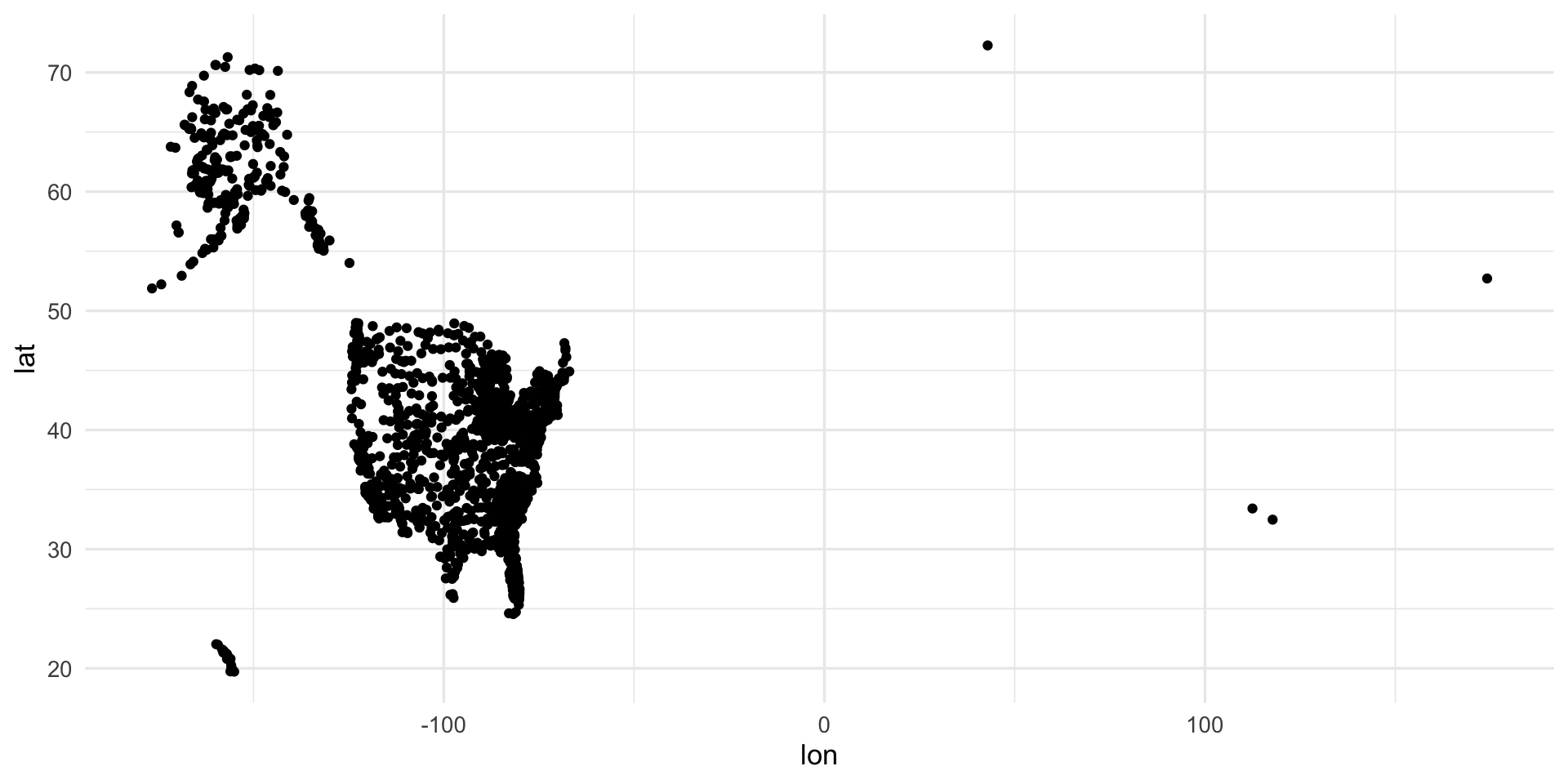
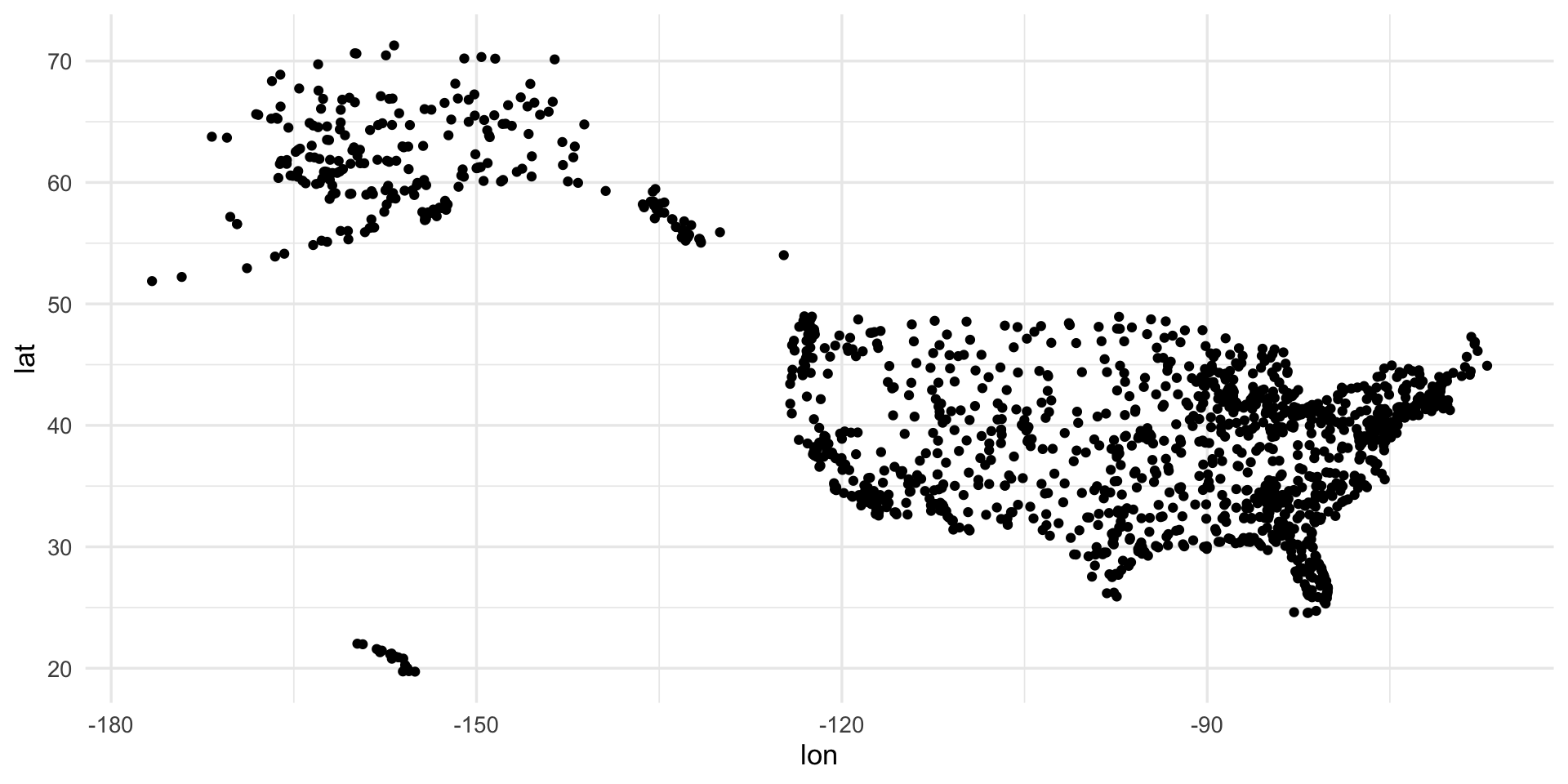
Error in UseMethod("show_query"): no applicable method for 'show_query' applied to an object of class "c('gg', 'ggplot')"

Take-away message

dbplyr is awesome and can often be helpful in figuring out SQL syntax
sometimes dbplyr will provide SQL syntax that does not work (see the median example)
sometimes there is no SQL syntax to match the R task of interest (see ggplot)

Best practice

It is always a good idea to terminate the SQL connection when you are done with it.

dbDisconnect(con_air, shutdown = TRUE)

47

Pomona’s number is 47, and I wanted to have a 47th slide.

icon that says STATS, DATA, MATH but has a 47 replacing every instance of AT in the words.'.

Figure 1: image credit: Jo Hardin

SQL Extras

Back to the flights

Efficiencies

KEYs

INDEXes

SHOW INDEXES

SHOW INDEXES

Partitioning

Querying quickly

EXPLAIN with distance

EXPLAIN with year

Cardinality x rows

EXPLAIN with year and month

EXPLAIN with month

EXPLAIN with JOIN - faster

EXPLAIN with JOIN - slower

SQL in dbplyr

Median

Median

Median

Median

Median

Median

Median

Median

Median

CASE WHEN and ifelse()

CASE WHEN and ifelse()

CASE WHEN and ifelse()

CASE WHEN and case_when()

CASE WHEN and case_when()

CASE WHEN and case_when()

CASE WHEN and cut()

CASE WHEN and cut()

CASE WHEN and cut()

distinct()

distinct()

distinct()

LIMIT as head()

LIMIT as head()

LIMIT as head()

ggplot()

ggplot()

ggplot()

Take-away message

Best practice

47

`KEY`s

`INDEX`es

`SHOW INDEXES`

`SHOW INDEXES`

`EXPLAIN` with `distance`

`EXPLAIN` with `year`

`Cardinality` x `rows`

`EXPLAIN` with `year` and `month`

`EXPLAIN` with `month`

`EXPLAIN` with `JOIN` - faster

`EXPLAIN` with `JOIN` - slower

`CASE WHEN` and `ifelse()`

`CASE WHEN` and `ifelse()`

`CASE WHEN` and `ifelse()`

`CASE WHEN` and `case_when()`

`CASE WHEN` and `case_when()`

`CASE WHEN` and `case_when()`

`CASE WHEN` and `cut()`

`CASE WHEN` and `cut()`

`CASE WHEN` and `cut()`

`distinct()`

`distinct()`

`distinct()`

`LIMIT` as `head()`

`LIMIT` as `head()`

`LIMIT` as `head()`

`ggplot()`

`ggplot()`

`ggplot()`